Math Development Program

Before we get into the “main course” for this issue, I would like to present a brief discussion of what “Simultaneous Linear Equations” are, for the benefit of those who may not be familiar with these concepts, or need to brush up a hazy memory from high-school or college days. It’s not intended as a course in S.L.E., as we just don’t have the space for such an undertaking. I do hope to give enough information to spur your interest to do as Mr. Bent suggests and bone up on the subject using a good text or even an outline book if all you need is a refresher.

Let’s start out with a simple mathematical relation expressed in words. Suppose someone told you he bought 20 apples and 5 mangos for $5.75. You could not deduce much about the price of apples and mangos as there is an infinite number of possibilities (assuming that fractional cent values are allowed). But suppose he also told you that had he bought 6 apples and 10 mangos it would have cost $6.40. Ah, now you can sit down with pencil and paper and figure out how much each costs. Before you read on, try to work out the solution to this little problem.

As it turns out, the word problem above can very easily be converted to algebraic equations (how convenient!).

20*X+5*Y = 5.75 and 6*X+10*Y = 6.40

where X is the price of apples and Y is the price of mangos.

This pair of equations is termed a “system” of equations. In order for both equations to hold true at the same time (hence “simultaneous”), the values for X and Y must “satisfy” both; i.e., when we plug them into either equation we should have both sides of the equal sign the same. Put the values you found into the equations as a check on your work; both equations should balance. (If you’ve forgotten how to solve this type of system, here’s a hint: multiply each term in the first equation by 2, then subtract the second equation term by term from the first. This results in an equation from which Y has been eliminated, and you should have no trouble finding X=.15 and then put that value back into either of the original equations and get Y=.55.)

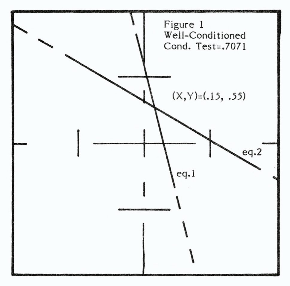
OK so far, but why “linear?” Linear means having to do with straight lines, and linear equations are ones that produce straight lines when graphed. As it turns out, this is only true of equations in which the variables are not raised to powers or have other functional operations (e.g. SIN, ATN, LN, etc.) performed on them. In this installment we will only deal with this type of system. If we graph our fruity problem above, we come up with a plot like Fig. 1. Line 1 represents all the combinations of x and y which satisfy the first equation, and line two is all the points which Satisfy the second. The point where they intersect is the solution – the only point which simultaneously satisfies both equations

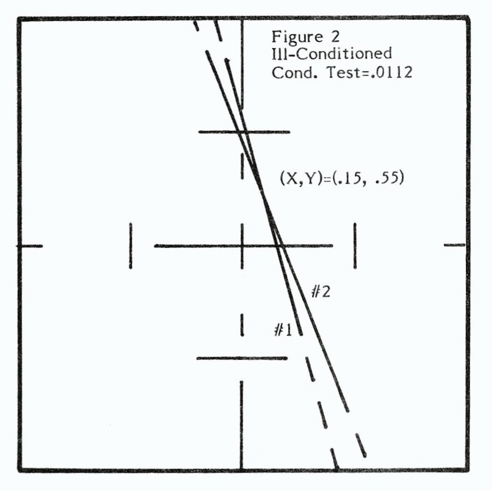
At this point, let’s assume that the second equation were 21*X + 5*Y = 5.90 instead. The system still gives the same solution, as you can verify. A graph of this modified system is shown in Fig, 2. Again there’s one discrete solution, but in this case the lines are very nearly parallel. Such a system is called “ill-conditioned,” and is less likely to give accurate results when using a computer. Just as it’s harder to discern the intersection point on the graph, so also the computer has difficulty resolving the exact solution. The program includes a routine that checks for ill-conditioning and yields a number between 0 (parallel lines or the same line and possessing no discrete solution) and 1 (perpendicular lines, and most accurate) to rate the system.

So big deal. We don’t need a computer to solve simple systems like this. The rub comes when we try to solve systems with more than two variables – try solving a six-variable system sometime! Note that for a solution we must have at least as many equations as we have unknowns, so you can see that things rapidly get out of hand. What we need is a systematic approach the computer can just crunch away at. Such systematic approaches were developed long before computers were, so don’t get the idea that all this is a new development. With a computer, though, even the huge task of solving 10th order S.E. becomes routine.

The first step is to convert our system of equations into an array called a matrix. Matrices are mathematical entities that can be operated on according to certain rules. Study Mr. Bent’s multiplication example to see why we can express our system as follows:

We thus have two arrays of numbers, one on either side of the equal sign, that specify the system. The matrix on the left side contains the multipliers (coefficients) of the unknowns, and the one on the right contains the constants each equation adds up to. For convenience, we can combine the two matrices into one 2×3 matrix, as this makes it easier to input the numbers. Just remember that the last column is the constants, the others are the coefficients.

Now that we have our matrix, we need some way to boil it down into answers. One way is by breaking it down into “determinants,” which is another form of array. Unlike a matrix, though, a determinant boils down to a single number, when evaluated according to certain simple rules, The bigger it is, the more calculations it takes, but you’ll always end up with a number that can be used to obtain a solution. To keep this distinction in view, we’ll indicate matrices with brackets, and determinants with straight lines. Arrays that are essentially a “butt-splice” of two matrices — Le, the way you input the numbers to the computer, are shown with curved brackets as they are neither matrices nor determinants but a shortcut for convenience. These will usually be N*N+1 in dimension.

I hope this has whetted your appetite for the article. A few short notes on the program: Enter RUN to start, push F or S for fast or slow mode. The main menu appears, options 1-3 allow matrix operations, 4 evaluates a determinant, and 5 goes on to the main S.L.E. portion. Selecting this gives an SE menu that is a veritable smorgasbord of possibilities. I particularly like combination plate #7, I think you will too. After completing analysis by Gauss Elimination and/or Gauss Seidel any size, you can repeat the problem using Cramers Rule by selecting 5, then 2, and pressing “N” on “NEW DATA” prompt. This is the only program I’ve seen allowing all three methods, even though CR any size “cheats” by using GE to do the dirty work. For this reason it usually gives the same results as GE (actually results ar more accurate, but the time scale is considerably larger), but I added it to demonstrate row-swapping of the last row with the others to get the determinants for each answer.

By Thomas Bent

First, a hearty hello to all you ZX/TSers out there! I would like to say a few words about myself before going too far. My computer background consists of a couple years of Basic and Fortran with Pascal as a new addition. For those of you familiar with DEC equipment, some Focal language also. My job doesn’t consist of a lot of programming, but the need to use a computer to solve problems for myself (and my boss) sent me in search of this programming tool. Since I do quite a bit of materials testing, I do a fair amount of set-up and program design on an assortment of computers. I am also a professional pilot holding a commercial, multi-engine rating.

Many of those who initially purchase the ZX/TS computer buy it with little knowledge of how computers work. Most of the rest, who know how they work, can’t afford anything more expensive. Then there are those who hold out for a more expensive computer simply because they can’t believe that a $30.00 computer can do what they want.

I have been pleasantly surprised with my Sinclair in the past two and a half years, and I look forward to a computerized world in which I know I will be able to hold up my end of the load. What I hope to do in a series of upcoming articles is to bring newcomers “up to speed” in some basic techniques of programming math routines on the ZX/TS, so that you won’t have to shy away from a project simply for a lack of knowledge on how to program these routines. Those who are familiar with this material can incorporate the routines into their own programs conveniently.

What I plan to cover will include but not be limited to more integration, numerical differentiation (polynomial and real-time,) curvefitting of various types, finding roots of equations, and simultaneous equations. Some of these techniques are hard to understand at first, but very easy to program. Please try to follow the development of the first subject, Simultaneous Linear Equations, because these routines will be used as subroutines in many programs that lie ahead.

Most high-school and college students know how to solve linear simultaneous equations (sim. eq.) and I’m sure they will agree that they have better things to do with their time. This first part will provide some useful programs for solving these types of problems, and will greatly speed up that engineering and/or math homework.

Before we start, let’s get one thing straight; all computers are notorious liars, Apple, Atari and VIC computers (6502 chip) do not handle floating point mathematics well. One reason that the ZX/TS is much slower when grinding numbers is because it has much better resolution (5-byte floating point as opposed to 4-byte for the others, or two extra decimal places accuracy). However if you want speed then you can always get a compiler (e.g. Bob Berch, 19 Jacques St., Rochester, NY 14620) and speed up those “integer” calculations anyway. REMEMBER!! There are many large holes in the computer number line and many numbers are stored inaccurately (e.g. Pi, .2, 1.3). This is quantizing error. Addition, subtraction, etc. are also done inaccurately (try taking the cube root [or square root] of eight, cube it [square it], and subtract 8 on your calculator). This is roundoff error, Heaven forbid you should add two inaccurate numbers many times and say, “the answer is….”!! One last point, if your data is accurate to two decimal places then your answer after several calculations certainly is no better. Throw away all those insignificant figures, they do you more harm than good.

Alright now, on with the show.

The good news is, this series will provide a complete computer math program and hopefully some understanding behind how the routines work. The bad news is that the material tends to be rather dry (and may require some WORK). The laughs will come later when you see how easy the homework becomes. The future chapters of this report will be integrated with this first section. I think if you should be very easy.

The Sim. Eq. techniques (S.E.) we will delve into this time around are Gauss-Seidel, Cramer’s Rule, and Gauss elimination, This is a tough subject to explain and to grasp, fortunately it is easier to program. It may require some extra homework, but if there are any questions don’t hesitate to write (this still holds-ed.) If S.E. are understood then many upcoming topics will be a snap.

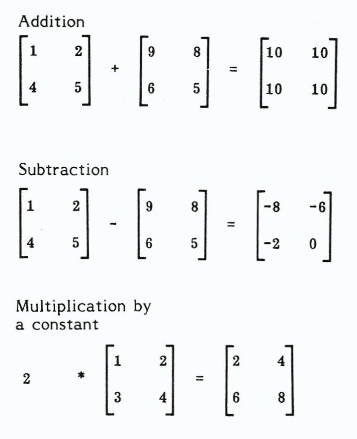
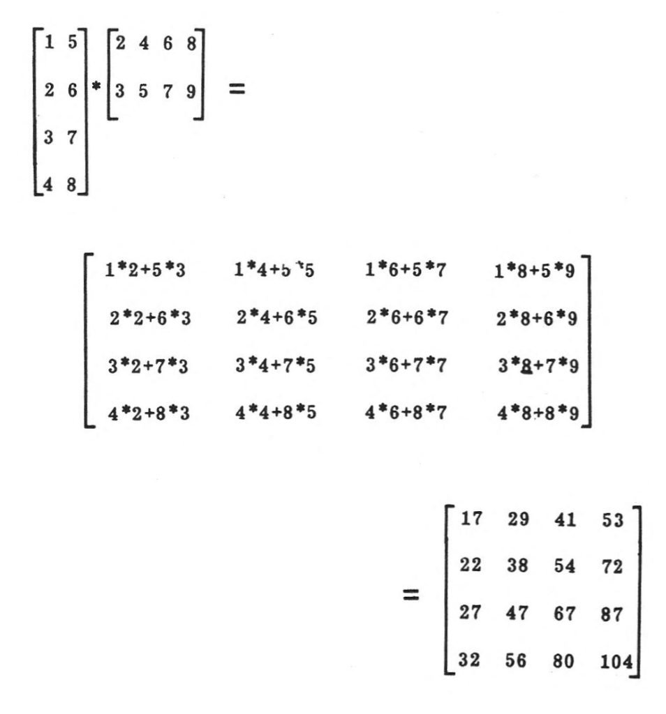
Manipulating matrices is the main scientific use of computers, You can add and subtract matrices of the same size, or multiply them by a constant. You can also multiply square or rectangular matrices where the number of columns. of the first matrix equals the number of rows of the second. Multiplying matrices is only tricky at first, but as you can see in the program, this is done with three loops and one calculation line, Please take the time to work through the given multiplication example so that the following S.E. routines will be more familiar and easier to debug.

You multiply rectangular matrices as follows:

A 4x2 * 2x4 = 4x4
A 2x4 * 4x2 = 2x2

I have worked out an example of the first case to show all the calculations involved. In the program, you input the size of matrix A and the computer only accepts input for the number of columns of matrix B. The product, matrix C has as many rows as A and as many columns as B.

It is much easier for the ZX/TS to do this kind of grunt work, and I think you’ll agree.

Determinants (det) are SQUARE arrays of any size, e.g. 2×2, 10×10, with some unique properties, A det is a single number in the form of an array of numbers, An Nth order det generates a predetermined number of calculations to solve, namely N factorial (N!) times (N-1). A 3rd order (3×3) det generates 12 calculations (3*2*1)*(3-1). A 10th order det generates 10!9 or in excess of 32,600,000 calculations! There are identities (det = 1) and inverse dets, among others. Please refer to a good math book or even flip through a Shaum’s outline book at your nearest book store for the properties of dets. Two important properties we must program for are:

1. If you interchange two rows of a det, the absolute value does not change, but the sign is reversed,
2. Adding one row of a det to another does not change the value of the determinant.

Evaluating a small det is easy and is done as follows:

In array form it looks like this:

Larger ones just get more cumbersome and tougher to keep straight.

The large det just gets broken down into smaller units and manipulated. By the way, if one row is a multiple of another row, the determinant = 0.

Taking what has just been discussed, we will transform our det (since we know some key properties) to reduce the astronomical number of calculations to something more manageable. In order to reduce round-off error, we should insure that the diagonal terms [A(1,1), A(2,2), etc.] contain the largest absolute value in their respective columns, for the terms below them. By this I mean that after evaluating col 1 row 1, leave that row alone [the col values below A(1,1) will all be zero.] Of course the last row gets whatever values are left.

What happens in the program is, the det is INPUT and col 1 is checked for the largest term. A zero term is checked for as this would mean an infinite number of solutions. The row with the largest value in col 1 is swapped with row 1. The new row 1 is multiplied by a different constant for each remaining row, so that every value in col 1 below the first term is zero when row 1 is subtracted from the row in question. Row 1 is now complete, as is col 1. Our “Pivot” now moves diagonally A(2,2), and the same trick is done again on the smaller array and so on until the last row (where there is only one term left). You must keep track of the number of times you swap rows (sign change) and simply multiply all of the diagonal terms together with the value of the sign (+ or -1) and voila! A 10×10 array takes less than 1000 calculations. A 6×6 array would not be uncommon for an engineer or engineering student. Most of us usually only see a 3×3 (because of the complexity and grunt work).

Simultaneous Equations (SE) will typically be 3×4 [or generally, Nx(N+1)] arrays and are handled much the same as determinants. Now we no longer have one number to deal with and must “back-calculate” the values that will solve the system of equations in question. The matrix is reduced the same way as the det is, except now we rearrange (put everything on the other side of the equality) our array to produce the values for X and Y [X(1) and X(2).]

The general form is:

AX + BY = E 
CX + DY = F

A, B, C, D, E and F are constants that are entered. X and Y we must solve for.

After reducing the matrix by multiplying row 1 by C/A and subtracting from the second row, the CX term cancels out and the second row becomes DY – CB/AY =F (the first row doesn’t change value.) The computer can quickly solve for Y and put that value in equation 1 and back out the value of X. There are no sign changes in SE to keep track of.

The computer will look for equations like this to solve for:

A(1,1) + A(1,2) + A(1,3) = A(1,4)
A(2,1) + A(2,2) + A(2,3) = A(2,4)
A(3,1) + A(3,2) + A(3,3) = A(3,4)

In the programs we dimension A(M,N) where M is the number of rows and N is the number of columns. This will give generality for any size array you have to solve for. X is dimensioned by M also, as linear SE are only valid for one unknown per equation. The computer will respond with one X for each column, that is, the answer for column 1 is X(1), etc. and that X is supposed to satisfy all M equations. (Hope and pray!)

Cramer’s Rule is very easy to program for small arrays (2×3), but gets tougher quickly thereafter. For 2 equations & 2 unknowns, in fact, it consists of only 3 program lines. Cramer’s Rule (CR) breaks the matrix into determinants (only one number) and solves for each unknown independently. This method is very close to how you solve linear SE by hand. Look at the following equations:

AX + BY = C
DX + EY = F

Multiply the top equation by E, the bottom equation by B and subtract the second equation from the first.

+(EAX + EBY = EC)
-(BDX + BEY = BF)
-----------------
EAX - BDX = EC - BF

Then consolidate X and solve.

X * (EA-BD) = EC-BF or
X = (EC-BF) / (EA - BD)

If this does not look familiar to you at this point, have no fear. We shall repeat the same thing again below the way the computer sees it.

AX + BY = C
DX + EY = F
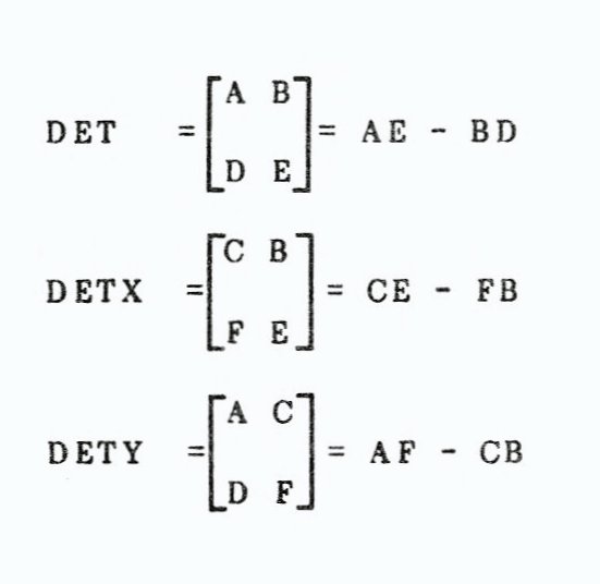
X = (C*E - B*F) / (A*E - B*D) and 
Y = (A*F - C*D) / (A*E - B*D) 
or,
X = (DET X) / (DET) 
Y = (DET Y) / (DET)

where

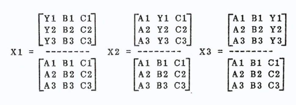
If you look back at the section on determinants, you should see the connection. The denominator is the same for both X and Y, and the numerator swaps terms. Watch that the-denominator is not zero as the solution is undefined. How this works is easy to see in a 3×4, but is tougher to program directly, as in the case of the 2×3.

Al + Bl + CI = Y1 
A2 + B2 + C2 = Y2 
A3 + B3 + C3 = Y3

The three answers are as follows:

I prefer Gauss Elimination when solving for any system of higher order than 2×3, as CR requires a lot more calculations (takes longer and accuracy suffers) and also requires more memory space.

This method is designed for a computer although it is an old technique. What it does is start with a guess at what the value is, plugs and chugs and goes back to the beginning with a new guess (the value it just solved for). Sounds great! Only one drawback; it doesn’t always work. However, we can stack the odds in our favor. Gauss-Seidel (GS) is guaranteed to work if the value of the diagonal terms are greater than the sum of the terms in the row plus the the sum of the terms in the column. Another way to help make this work will be to begin with a different starting value if necessary. GS is very memory efficient and is not susceptible to round-off error like the other techniques. Each iteration is just like starting over, if the present answer is not good enough then go back and try again. You can also watch the computer approach the answer rather than sitting and waiting.

Should GS diverge or jump around, simply BREAK in and assign X values directly (LET X(1) = -10 or some other value), then CONT to see if that helps. If that doesn’t work, then BREAK and RETURN to try another way. Initially all X values will be assigned zero. The equations are swapped using the GE subroutine (but not reduced), unless you input the equations in the proper order, in which case the subroutine can be bypassed (saving memory), The computer will manipulate the equations to simulate the following:

AX(1) + BX(2) = C 
DX(1) + EX(2) = F
Then,
X(1) = (C - BX(2)) / A 
X(2) = (F - DX(1)) / E 
and so on.

Actually, the X term being evaluated is on both sides of the equation, but is assigned to zero every time through the loop. There must be an outside loop controlling the maximum number of iterations in case of divergence. Normally, 30 iterations will be more than enough for 6-place accuracy, but 100 may be necessary depending on how ill-conditioned the system of equations is (see the graphs).

To test for ill-conditioning, you “normalize” the determinant of the system of equations. This means that you square each term in the row, add them up and divide each term in the row by the sum of the squares (more on this next time), GOSUB GE to evaluate the determinant and you have a number less than one. If it is less than .2 then you may have trouble trying to solve your SE by any other method than by hand (but not necessarily). If you are concerned about the accuracy of your answers then try changing your matrix slightly and see if your answers vary largely, If so then get out your pencil and paper.

10 REM SE VERSN 3.2 4/1/84
34 GOTO 1000
38 REM INPUT DATA POINTS
42 PRINT "HOW MANY POINTS?"
46 INPUT M
50 LET DP=M
54 DIM P(M)
58 DIM U(M)
62 DIM V(M)
66 DIM Y(M)
70 PRINT " INPUT X THEN Y VAL"
74 FAST
78 FOR I=A TO M
82 PRINT TAB TR;I;" ";
86 INPUT P(I)
90 INPUT Y(I)
94 PRINT P(I),Y(I)
98 IF I>18 THEN GOSUB 910
102 NEXT I
106 GOTO 666
110 PRINT ,," INPUT START / STOP FOR X THEN Y"
114 DIM E(D)
118 DIM E$(D,D)
122 FOR I=A TO D
126 IF I=A OR I=TR THEN PRINT ("X  " AND I=A)+("Y  " AND I=TR)
129 INPUT E$(I)
134 PRINT E$(I),
138 NEXT I
142 RETURN
146 FOR I=A TO D
150 LET E(I)=VAL E$(I)
154 NEXT I
158 RETURN
162 PRINT ,," INPUT TITLE";
166 INPUT T$
170 PRINT T$
174 PRINT ,," INPUT X LABEL";
178 INPUT X$
182 PRINT X$
186 PRINT ,," INPUT Y LABEL";
190 INPUT Y$
194 PRINT Y$
198 RETURN
202 PRINT ,," INPUT X LOG/LIN 1/0"
206 INPUT XL
210 PRINT ,," INPUT Y LOG/LIN 1/0"
214 INPUT YL
218 RETURN
222 LET E(A)=LN E(A)/K
226 LET E(TW)=LN E(TW)/K
230 RETURN
234 LET E(TR)=LN E(TR)/K
238 LET E(D)=LN E(D)/K
242 RETURN
246 REM PLOT SETUP
250 DIM O(M)
254 DIM Q(M)
258 CLS
262 PRINT "LABEL GRAPH? 1/0 ES=1 NO=0"
266 INPUT SL
270 IF SL THEN GOSUB 162
274 CLS
278 PRINT ,,"SET SCALE? 1/0 NO=0"
282 INPUT SS
286 IF SS THEN GOSUB 202
290 PRINT ,,"SET HIGH/LOW LIMIT? 1/0 NO=0"
294 INPUT SSL
298 IF SSL THEN GOSUB 110
302 PRINT ,,"POINTS CONNECTED? 1/0 NO=0"
306 INPUT CN
310 PRINT "PLOT CURVE FIT? 1/0 NO=0"
314 INPUT CF
318 PRINT ,,"LIMITS OK? 1/0 NO=0"
322 INPUT Z
326 CLS
330 IF NOT Z THEN GOTO 246
338 GOSUB 146
342 LET K=LN 10
346 IF NOT XL THEN GOTO 366
350 GOSUB 222
354 FOR I=A TO M
358 LET U(I)=LN P(I)/K
362 NEXT I
366 IF XL THEN GOTO 382
370 FOR I=A TO M
374 LET U(I)=P(I)
378 NEXT I
382 IF NOT YL THEN GOTO 402
386 GOUB 234
390 FOR I=A TO M
394 LET V(I)=LN Y(I)/K
398 NEXT I
402 IF YL THEN GOTO 418
406 FOR I=A TO M
410 LET V(I)=Y(I)
414 NEXT I
418 REM PLOT NOW
422 LET DX=(E(TW)-E(A))/56
426 LET DY=(E(D)-E(TR))/40
430 LET PL=A
434 FOR I=A TO M
438 LET TX=(U(I)-E(A))/DX
442 IF TX<ZO OR TX>57 THEN GOTO 466
446 LET TY=(V(I)-E(TR))/DY
450 IF TY<ZO OR TY>40 THEN GOTO 466
454 LET O(PL)=INT (TX+7.5)
458 LET Q(PL)=INT (TY+3.5)
462 LET PL=PL+A
466 NEXT I
470 FOR I=TR TO 63
474 IF I<44 THEN PLOT 6,I
478 IF I>5 THEN PLOT I,TW
482 NEXT I
486 IF NOT SL THEN GOTO 518
490 LET T=10-LEN Y$/TW
494 FOR I=A TO LEN Y$
498 PRINT AT T,A;Y$(I)
502 LET T=T+A
506 NEXT I
514 PRINT AT 21,16-LEN X$/TW;X$
518 PRINT AT 21,TR;E$(A);AT 21,28;E$(TW)
522 PRINT AT ZO,ZO;E$(D, TO TR);AT 20,ZO;E$(TR, TO TR)
526 SLOW
530 FOR I=A TO PL-A
534 PLOT O(I),Q(I)
538 NEXT I
542 IF NOT CF THEN GOTO 558
546 FOR I=A TO PF-A
550 PLOT F(I),G(I)
554 NEXT I
558 IF NOT CN THEN GOTO 622
562 FOR I=A TO PL-TW
566 LET Q=Q(I+A)-Q(I)
570 LET O=O(I+A)=O(I)
574 IF O=ZO THEN GOTO 618
578 LET T=Q/O
582 IF ABS T>A THEN GOTO 606
586 LET J=Q(I)=T*O(I)
590 FOR L=O(I) TO O(I+A)-A STEP SGN O
594 PLOT L,L*T+J
598 NEXT L
602 GOTO 618
606 FOR L=Q(I) TO Q(I+A)-A STEP SGN Q
610 PLOT (L+T*O(I)-Q(I))/T,L
614 NEXT L
618 NEXT I
619 IF NOT SL THEN GOTO 622
620 POKE 16418,ZO
621 PRINT AT 21,27;,TAB 16=LEN T$/TW;T$
622 FOR I=A TO PL-A
626 UNPLOT O(I),Q(I)
630 PLOT O(I),Q(I)
634 IF INKEY$<>"" THEN GOTO 646
638 NEXT I
642 GOTO 622
646 IF INKEY$<>"Z" THEN GOTO 666
650 COPY
654 IF SL THEN LPRINT T$
658 IF CF THEN LPRINT ,,"THE FUNCTION IS:",F$
662 IF CF THEN LPRINT ,,"THE CORRELATION COEFFICIENT IS:",R
664 IF CF THEN LPRINT ,,"THE RESIDUALS:",,"SUM OF Y",RY,"SUM OF XY,",RXY
666 CLS
667 POKE 16418,2
670 SLOW
674 PRINT "WOULD YOU LIKE TO:",,,"0. RETURN TO MAIN MENU","1. PLOT (RESCALE?)","2. (RE)FIT DATA",,"3. RESCALE FIT",,"4. PRINT VALUES"
678 INPUT Z
682 GOTO (722 AND(Z=TR OR Z=D)+(1000 AND NOT Z)+(246 AND Z=A)+(686 AND Z=TW)
686 CLS
690 PRINT "WHICH TYPE OF FIT?",,,"0. INTERPOLATION",,,"LEAST SQUARES FIT (REGRESSION):",,,"1. LINEAR",,"2. EXPONENT",,"3. LOGARITHMIC",,"4. POWER",,,,"5. POLYNOMIAL"
694 INPUT Z
698 IF Z AND Z<5 THEN GOTO 714
702 IF NOT Z OR Z=5 THEN PRINT ,,"WHICH DEGREE?","ENTER",,,("** 1 LINE " AND NOT Z),("2 PT." AND NOT Z),"**2 PARABOLA","3","**3 CUBIC","4","**INPUT ","N-1"
706 INPUT DEG
710 CLS
714 GOSUB (4980 AND Z)+(4400 AND NOT Z)
718 GOTO 666
722 GOSUB (5540 AND Z=TR)+(4000 AND Z=D)
726 CLS
730 IF Z=TR THEN PRINT "FIT RESCALE DONE",,,
734 GOTO 667
910 SCROLL
920 PRINT AT 21,31;" ";AT 21,ZO;
930 RETURN
940 CLEAR
950 FAST 960 FOR I=1 TO 22
970 SCROLL
980 NEXT I
990 SAVE "SE"
997 LET F$=""
999 REM FLAGS NUMBERS ETC
1000 LET ZO=NOT PI
1001 LET A=NOT ZO
1002 LET TW=A+A
1003 LET TR=TW+A
1004 LET D=TR+A
1006 LET AL=ZO
1007 LET LS=ZO
1010 LET CR=NOT PI
1012 LET IP=CR
1020 LET DE=CR
1030 LET GS=DE
1040 LET S=A
1050 LET IL=DE
1059 CLS
1060 SLOW
1070 PRINT TAB 5;"---COMPUTER MATH---",TAB 5;"DEVELOPMENT PROGRAM",,"BY THOMAS BENT",,,OPTIONS:"
1080 PRINT ,,"0) STOP ",,"1) ADD 2 MATRICES","2) SUBTRACT 2 MATRICES","3) MULTIPLY 2 MATRICES","4) EVALUATE A DETERMINANT","5) SIMULTANEOUS LIN. EQUATIONS","6) PRINT / PLOT AND FIT DATA","7) INTEGRATION"
1090 INPUT Z
1100 CLS
1110 IF NOT Z THEN STOP
1120 GOTO (5998 AND Z=7)+(1160 AND Z=5)+(38 AND Z=6)+(1130 AND Z<5)
1130 GOSUB (2730 AND Z<TR)+(2950 AND Z=TR)+(3200 AND Z=D)
1140 SLOW
1150 GOTO 1220
1160 PRINT ,,"WHICH METHOD TO USE?"
1170 PRINT ,,"1. CRAMERS RULE 2X3","2. CRAMERS RULE ANY SIZE","3. GAUSS ELIMINATION ANY SIZE","4. GAUSS SEIDEL ANY SIZE","5. COMPARE NO. 3 AND 4","6. CHECK FOR ILL-CONDITIONING","7. COMBINATION 5,6","8. COMBINATION 3,6"
1180 INPUT Z
1190 CLS
1200 GOSUB (3680 AND Z=TS)+(1350 AND Z=D+D)+(1310 AND Z=D+TR)(1270 AND Z=D+A)+(2620 AND Z=A)+(1730 AND Z=TR)+(2200 AND Z=D)+(3350 AND Z=D+TW)
1210 SLOW
1220 IF INKEY$="" THEN GOTO 1220
1230 FAST
1240 IF INKEY$="Z" THEN COPY
1250 REM YOUR SCREEN DUMP HERE
1260 GOTO 1000
1270 REM 5
1280 GOSUB 2200
1290 GOSUB 1750
1300 RETURN
1310 REM 7
1320 GOSUB 2200
1330 GOTO 1360
1340 REM 8
1350 GOSUB 1400
1360 GOSUB 3350
1370 GOSUB 1750
1380 GOSUB 3500
1390 RETURN
1400 REM INPUT DATA
1420 PRINT ,,"HOW MANY ROWS FOR ""A""? ";
1430 INPUT M
1440 PRINT M
1450 PRINT ,,"HOW MANY COLS? ";
1460 INPUT N
1470 PRINT N
1480 DIM A(M,N)
1490 DIM Z(M,N)
1495 FAST
1500 FOR I=A TO M
1510 GOSUB 910
1520 PRINT AT 20,ZO;"ROW COL","VAL ",I;
1530 FOR J=A TO N
1540 PRINT TAB D;J,
1550 INPUT A(I,J)
1560 PRINT A(I,J)
1570 LET Z(I,J)=A(I,J)
1580 GOSUB 910
1590 NEXT J
1600 NEXT I
1610 CLS
1620 RETURN
1630 REM RECALL AREA A
1640 DIM A(M,N)
1650 FAST
1660 FOR I=A TO M
1670 FOR J=A TO N
1680 LET A(I,J)=Z(I,J)
1690 NEXT J
1700 NEXT I
1710 SLOW
1720 RETURN
1730 REM GAUSS ELIMINATION
1740 GOSUB 1400
1750 DIM X(M)
1760 REM SWAP ROWS
1770 FAST
1780 FOR I=A TO M-A
1790 LET B=ZO
1800 FOR J=I TO M
1810 LET P=ABS A(J,I)
1820 IF P>B THEN LET L=J
1830 IF P>B THEN LET B=P
1840 NEXT J
1850 IF NOT B THEN STOP
1860 IF IL OR I=L THEN GOTO 1930
1870 LET S=-S
1880 FOR J=A TO N
1890 LET T=A(I,J)
1900 LET A(I,J)=A(L,J)
1910 LET A(L,J)=T
1920 NEXT J
1930 IF GS THEN NEXT I
1940 IF GS THEN RETURN
1950 REM REDUCE
1960 LET NLINE=I+A
1970 FOR J=NLINE TO M
1980 LET C=A(J,I)/A(I,I)
1990 FOR K=I TO N
2000 LET A(J,K)=A(J,K)=C*A(I,K)
2010 NEXT K
2020 NEXT J
2030 NEXT I
2040 IF DE OR IL THEN RETURN
2050 REM BACK SUB
2060 FOR I=M TO A STEP -A
2070 LET BK=A(I,N)
2080 IF I=M THEN GOTO 2120
2090 FOR J=M TO I STEP -A
2100 LET BK=BK-A(I,J)*X(J)
2110 NEXT J
2120 LET X(I)=BK/A(I,I)
2130 NEXT I
2135 IF IP THEN RETURN
2140 PRINT ,," RESULTS BY GAUSS ELIMINATION:"
2150 SLOW
2160 FOR I=A TO M
2170 PRINT TAB D;"X ";I,X(I)
2180 NEXT I
2190 RETURN
2200 REM GAUSS SEIDEL
2210 PRINT " INPUT ACCURACY DESIRED"
2220 INPUT ER
2230 CLS
2240 GOSUB 1400
2250 LET GS=A
2260 PRINT AT 19,D;"GAUSS SEIDEL ITERATIONS"
2270 GOSUB 1760
2280 LET GS=NOT GS
2290 DIM X(M)
2300 DIM Y(M)
2310 FAST
2320 FOR K=A TO 100
2330 GOSUB 910
2340 FOR I=A TO M
2350 LET T=ZO
2360 LET X(I)=T
2370 FOR J=A TO M
2380 LET T=T+A(I,J)*X(J)
2390 NEXT J
2400 LET X(I)=(A(I,N)-T)/A(I,I)
2410 NEXT I
2420 LET T=ZO
2430 PRINT K;
2440 FOR I=A TO M
2450 PRINT TAB D;"X ";I,X(I)
2460 GOSUB 910
2470 LET Y(I)=X(I)-Y(I)
2480 IF ABS Y(I)<=ER THEN LET T=T+A
2490 LET Y(I)=X(I)
2500 NEXT I
2510 PAUSE 100
2520 IF T<>M THEN GOTO 2580
2530 CLS
2540 PRINT ,,"GAUSS SEIDEL CONVERGED","IN ";K;" ITERATIONS, RESUTLS ARE:"
2550 GOSUB 2160
2560 SLOW
2570 RETURN
2580 NEXT K
2590 PRINT "GAUSS SEIDEL DID NOT CONVERGE"
2600 SLOW
2610 RETURN
2620 REM CRAMERS RULE
2630 LET M=TW
2640 LET N=TR
2650 GOSUB 1480
2660 LET CR=A(A,A)*(TW,TW)-A(TW,A)*A(A,TW)
2670 IF NOT CR THEN GOTO 3990
2675 DIM X(M)
2680 LET X(A)=(A(A,TR)*A(TW,TW)-A(TW,TR)*A(A,TR))/CR
270 PRINT ,,"RESULTS BY CRAMERS RULE ARE"
2710 PRINT ,,"X= ";X(A),"Y= ";X(TW)
2720 RETURN
2730 REM = OR =
2740 GOSUB 1400
2750 PRINT " INPUT MATRIX ""B"""
2760 DIM B(M,N)
2770 FOR I=A TO M
2780 PRINT " INPUT ROW ";I
2790 FOR J=A TO N
2800 INPUT B(I,J)
2810 NEXT J
2820 NEXT I
2830 CLS
2840 DIM C(M,N)
2850 PRINT "ROW COL";TAB 13;"MATRICES"
2860 PRINT "I   J";TAB 9;"A";TAB 16;"B";TAB 25;"C"
2870 FOR I=A TO M
2880 FOR J=A TO N
2890 IF Z=A THEN LET C(I,J)=A(I,J)+B(I,J)
2900 IF Z=TW THEN LET C(I,J)=A(I,J)-B(I,J)
2910 PRINT I;TAB D;J;TAB TR*TR;A(I,J);TAB D*D;B(I,J);TAB 25;C(I,J)
2920 NEXT J
2930 NEXT I
2940 RETURN
2950 REM MULTIPLY
2960 GOSUB 1400
2970 PRINT "HOW MANY COLS FOR B? "
2980 INPUT P
2990 DIM B(N,P)
3000 FOR I=A TO N
3010 PRINT " INPUT ROW ";I
3020 FOR J=A TO P
3030 INPUT B(I,J)
3040 NEXT J
3050 NEXT I
3060 CLS
3070 DIM C(M,P)
3080 FOR I=A TO M
3090 FOR J=A TO P
3100 FOR K=A TO N
3110 LET C(I,J)=C(I,J)+A(I,K)*B(K,J)
3120 NEXT K
3130 NEXT J
3140 FOR J=A TO P
3150 PRINT C(I,J);"     ";
3160 NEXT J
3170 PRINT
3180 NEXT I
3190 RETURN
3200 REM DETERMINANT
3210 GOSUB 1400
3220 LET DE=A
3230 GOSUB 1760
3240 LET DE=NOT DE
3250 FOR I=A TO M
3260 LET S=S*A(I,I)
3270 NEXT I
3280 IF CR THEN RETURN
3290 PRINT "THE DETERMINANT = ";S
3300 RETURN
3310 GOSUB 1400
3320 LET GS=NOT GS
3330 GOSUB 1760
3340 LET GS=NOT GS
3350 REM ILL-CONDITIONING
3360 DIM C(M,M)
3370 FOR I=A TO M
3380 LET T=ZO
3390 FOR J=A TO M
3400 LET C(I,J)=A(I,J)
3410 LET T=T+C(I,J)*C(I,J)
3420 NEXT J
3430 LET T=SQR T
3440 FOR J=A TO M
3450 LET C(I,J)=C(I,J)/T
3460 NEXT J
3470 NEXT I
3480 IF Z=D+TW THEN GOTO 3510
3490 RETURN
3500 REM 00
3510 FOR I=A TO M
3520 FOR J=A TO M
3530 LET A(I,J)=C(I,J)
3540 NEXT J
3550 NEXT I
3560 LET N=M
3570 LET IL=NOT IL
3580 GOSUB 1760
3590 LET N=M+A
3600 LET IL=NOT IL
3610 FOR I=A TO M
3620 LET S=ABS (S*A(I,I))
3630 NEXT I
3640 PRINT ,,"ILL CONDITIONING TEST ";
3650 IF S<A/D THEN PRINT " THE SYSTEM IS ILL CONDITIONED"
3660 IF S>=A/D THEN PRINT " THE SYSTEM IS OK"
3670 RETURN
3680 REM OR1
3690 PRINT " INPUT NEW DATA? Y=1 N=0"
3700 INPUT X
3710 IF X THEN GOSUB 1400
3720 LET CR=A
3730 CLS
3740 GOSUB 1630
3750 LET N=M
3760 FAST
3770 GOSUB 3220
3780 LET DEN=S
3790 PRINT "DENOMINATOR= ";S
3800 IF NOT S THEN GOTO 3990
3810 DIM X(M)
3820 FOR V=A TO M
3830 LET S=A
3840 LET N=M+A
3850 GOSUB 1630
3860 FOR U=A TO M
3870 LET A(U,V)=A(U,N)
3880 NEXT U
3890 LET N=M
3900 GOSUB 3220
3910 LET X(C)=S/DEN
3920 NEXT V
3930 LET N=M+A
3940 LET CR=NOT PI
3950 SLOW
3960 PRINT ,,"RESULTS BY CR:"
3970 GOSUB 2160
3980 RETURN
3990 PRINT "NO SOLUTION BY CR"
3995 RETURN