
Curve-plotting has many applications. For example, an oscilloscope is a curve-plotting device which allows the user to view time-varying voltages. This article presents a program which allows the Timex/Sinclair computers to be used as curve-plotting devices. The common representations of curves possible with this program include the following: Cartesian, Cartesian Parametric, polar, and polar parametric. An example of a polar plot would be the radiation pattern of an antenna. The program requires the 8K ROM and makes use of pixel graphics.
An Introduction to Curves
A plane curve is a two-dimensional path or set of points. Plane curves are found in such everyday places as the path followed by an ant on the kitchen floor or a magazine article on inflation. They can also be found in special places such as an oscilloscope trace or the spirals of a sunflower.
A plane curve can be described mathematically in various ways. A description which is adquate must be useful for the particular application at hand. For example, if the application is target shooting, it is only necessary to know whether a given trajectory passes through the bull’s-eye. Since the application addressed in this article is curve-plotting using the ZX81, an adequate description would tell which pixels the curve passes through. This description will be used to construct a display file which in turn will be used to display the plot of the curve.
Many curves can be described most concisely by the use of one or more equations. The equations can then be used to generate points of the curve. The curve-plotting program in this article operates by creating levels of descriptions of the curve as shown in Figure 1.
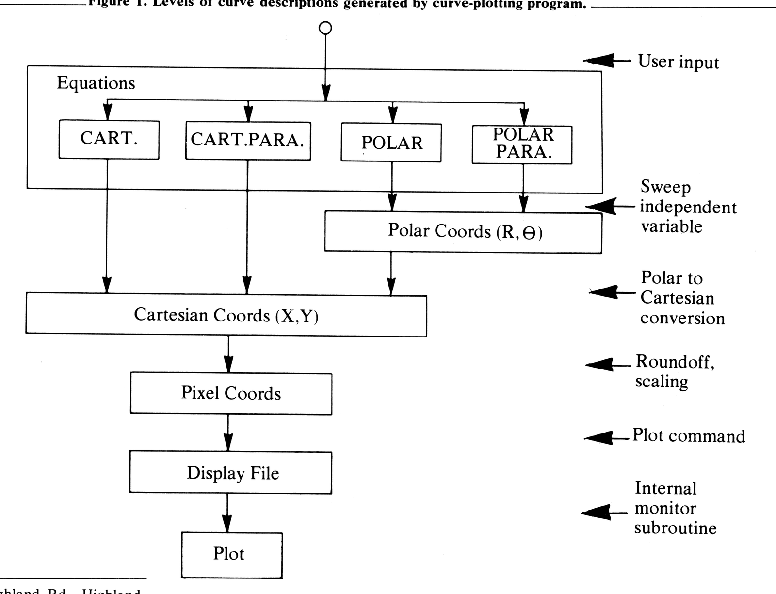
A point is located with respect to some reference system. There are no requirements upon the position or scale of the reference system itself so a convenient location and scale may be chosen. A Cartesian reference system is an X-Y axis. A polar reference system is a ray. In the Cartesian reference system a point is described by the coordinates (X,Y) of X and Y intercepts. In a polar reference system, a point is described by the coordinates (R, Θ ),where R is the length of the line segment between the base of the ray to the point and Θ (theta) is the angle between the line segment and the ray. Figure 2 shows the plot of a curve containing the point
(Rp Θp)
The positive X-axis of a Cartesian reference system coincides with the polar reference system. In this Cartesian reference system the point is described by
(Xp ,Yp ) = (Rp cosΘp , Rp sinΘp )
The curve-plotting program converts polar coordinates to Cartesian coordinates in this way to make use of the pixel graphics.
The methods used by the program to generate point coordinates make use of functional equations. A functional equation is one which evaluates some variable uniquely when the independent variable is given. This is expressed
VD = f(VI )
where VD is the dependent variable and VI is the independent variable.
The four approaches are best summarized in tabular form. See Figure 3.
To generate point coordiates, the independent variable is swept through a range of values and coordinates are calculated for values in the range.
Each type of description has its own advantages. For example, to generate a plot of a circle would take two sweeps of the independent variable using the Cartesian method, but only one sweep using the Cartesian parametric or polar methods.
Program Description
The program is listed in Figure 4. Lines 10-220 are used to input equations, plotting window, etc. Lines 220-350 generate the plot. Note that expressions are entered as string variables so that no program lines need to be changed for different plottings.
Also note in line 340 how points are scaled to pixel coordinates. Lines 300-330 remove points which are outside the plotting window.
Line 230 provides for 200 iterations of the FOR-NEXT loop. The number of iterations can, of course, be changed when necessary.
Program Use
The program first prompts the user with “CART., CART.PARA., POLAR, OR POLAR PARA.? (1,2,3, OR 4)”. Enter the number corresponding to the plot you want. For example, for Cartesian plots, enter 1. Next, a plotting window is entered. This is the expected region which will be covered in Cartesian space. See Figure 5.
If CART.PARA., POLAR, or POLAR PARA. was selected, a range must be entered for the parameter T or for theta, for example, an expression like PI/2.
When entering expressions for X, Y, R or theta, be sure to use expressions of the appropriate independent variable: For Cartesian plots use X; for all the others use T. Be careful when using expressions involving powers, since powers of negative numbers are not valid on the ZX80/81. For example, when X is negative, use X*X instead of X**2.
Sample Curves
To illustrate the program, several interesting curves may be used. Two examples of each of the following types are given. The reader can get further variety by changing the constants. Many more examples of curves can be found in A Catalog of Special Plane Curves by J. Dennis Lawrence (Dover Publications, 1972).

Figure 4. Curve-plotting program listing.
  20 PRINT "CART., CART. PARA., POLAR, OR POLAR PARA.? (1,2,3, OR 4)"
  30 INPUT Z
  40 PRINT "PLOTTING WINDOW:"
  50 PRINT " INPUT XMIN,XMAX,YMIN,YMAX"
  60 INPUT A
  70 INPUT B
  80 INPUT C
  90 INPUT D
 100 LET E=A
 110 LET F=B
 120 IF Z=1  THEN GOTO 200
 130 PRINT "PARAMETER/THETA RANGE:"
 140 PRINT " INPUT MIN,MAX"
 150 INPUT E
 160 INPUT F
 170 IF Z=3 THEN GOTO 200
 180 PRINT " INPUT X/THETA EXPRESSION"
 190 INPUT A$
 200 PRINT " INPUT Y/R EXPESSION"
 210 INPUT B$
 220 CLS
 230 FOR T=E TO F STEP (F-E)/200
 240 LET X=T
 250 IF Z=2 OR Z=4 THEN LET X=VAL A$
 260 LET Y=VAL B$
 270 IF Z<3 THEN GOTO 300
 275 LET W=X
 280 LET X=Y*COS W
 290 LET Y=Y*SIN W
 300 IF X<A THEN LET X=A
 310 IF X>B THEN LET X=B
 320 IF Y<C THEN LET Y=C
 330 IF Y>D THEN LET Y=D
 340 PLOT (X-A)*60/(B-A),(Y-C)*40/(D-C)
 350 NEXT T
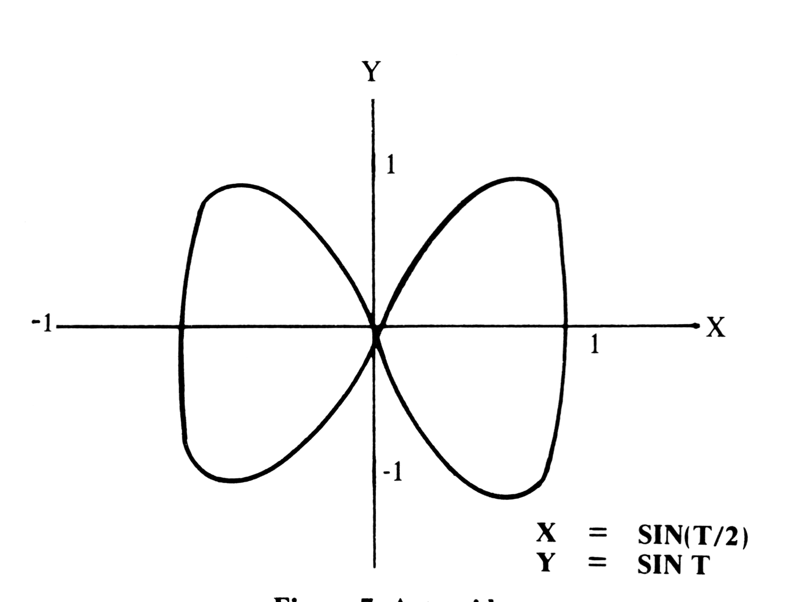
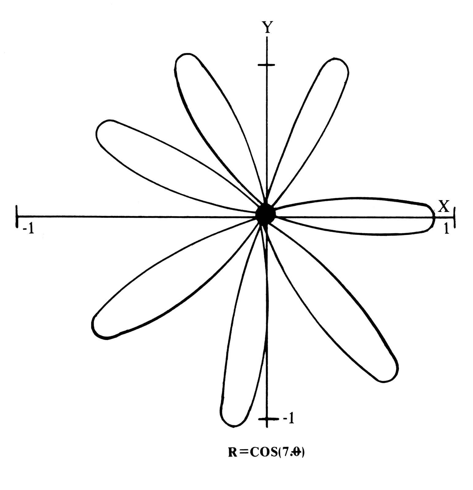
1. Lissajous Patterns. (See Figure 6.) a. General form: X=A*SIN(N*T+D) Y=B*SIN T b. This example: A=B=1; D=0 ; N=.75 c. Program data: ENTER: CART.PARA. 2 XMIN,XMAX,YMIN,YMAX -1,1,-1,1 PARAMETER RANGE -20,20 X EXPRESSION SIN (.75*T) Y EXPRESSION SIN T 2. Astroid. (See Figure 7.) a. General form: X=4*A*(COS T)**3 Y=4*A*(SIN T)**3 b. This example: A=.25 c. Program data: ENTER: CART.PARA. 2 XMIN,XMAX,YMIN,YMAX -1,1,-1,1 PARAMETER RANGE -PI,PI X EXPRESSION COS T*COS T*COS T Y EXPRESSION SIN T*SIN T*SIN T 3. Limacon of Pascal. a. General form: R=2*ACOS T+B b. This example: A=B=1 c. Program data: ENTER: POLAR 3 XMIN,XMAX,YMIN,YMAX -.5,3,-2,2 THETA RANGE -PI,PI R EXPRESSION 2*COS T+1 4. Rhodonea. (Figure 8.) a. General form: R=A*COS (N*T) b. This example: A=1; N=7 c. Program data: ENTER: POLAR 3 XMIN,XMAX,YMIN,YMAX -1,1,-1,1 THETA RANGE -PI,PI R EXPRESSION COS (7*T) 5. Serpentine. (Figure 9. a. General form: Y=X*B**2/(X**2+A**2) b. This example: A=2; B=6 c. Program data: ENTER: CART. 1 XMIN,XMAX,YMIN,YMAX -10,10,÷10,10 PARAMETER RANGE Y EXPRESSION (X*36)/(X*X+4) 6. Catenary. a. General form: Y=A/2*(EXP(X/A)+EXP(-X/A)) b. This example: A=2 c. Program data: ENTER: CART. 1 XMIN,XMAX,YMIN,YMAX -5,5,0,20 Y EXPRESSION EXP (X/2)+EXP (-X/2) 7. Eight Curve. a. General forms: THETA=ATN SIN T R=A*COS T*SQR (1+SIN T**2) b. This example: A=2 c. Program data: ENTER: POLAR PARA. 4 XMIN,XMAX,YMIN,YMAX -2,2,-2,2 PARAMETER RANGE -PI,PI THETA EXPRESSION ATN SIN T R EXPRESSION 2*COS T*SQR (1+SIN T*SIN T) 8. Folium of Descartes. a. General forms: THETA ATN T R=3*A*T*SQR (1+T**2)/(1+T**3) b. This example: A=5 c. Program data: ENTER: POLAR PARA. 4 XMIN,XMAX,YMIN,YMAX -10,10,-10,10 PARAMETER RANGE -5,5 THETA EXPRESSION ATN T R EXPRESSION 15*T*SQR (1+T*T)/(1+T*T*T) 9. Additional Examples: a. Polynomial (CART.): Y=A0+A1*X+A2*X**2+A3*X**3++AN*X**N b. Hypotrochoid (CART.PARA.): X=N*COS T+H*COS (N*T/B) Y=N*SIN T-H*SIN (N*T/B) c. Epitrochoid (CART.PARA.): X=N*COS T-H*COS (N*T/B) Y=N*COS T-H*COS (N*T/B) d. Archimedes' Spiral (POLAR): R=A*T e. Spirals (POLAR PARA.): THETA=T**M R=A*T
Figure 3.

Method        Independent   Coordinates               Example
              Variable
CARTESIAN     X             (X,Y) = (X,f(X))          Y=X**2 (PARABOLA)
CARTESIAN     T             (X,Y) = (f1(T),f2(T))     X=T (PARABOLA)
PARAMETRIC                                            Y=T**2
POLAR         THETA, or θ   (R,θ) = (f(θ),θ)          R=2*THETA (SPIRAL)
POLAR         T             (R,θ = (f1(T),f2(T))      THETA=T (SPIRAL)
PARAMETIC                                             R=2*T



Note: Type-in program listings on this website use ZMAKEBAS notation for graphics characters.