Solving Implicit Functions on the ZX81

Solving arithmetic and algebraic problems on the ZX81 is easy when the variable wanted is defined explicitly, that is, if you know that Y = X ** 2 + 2 * X, it is easy to program:

10 INPUT X
20 LET Y=X**2+2*X
30 PRINT Y

Now you put in the values of X and let the computer find the corresponding values of Y.

The fun begins when the variable you want is defined as an implicit function. Suppose, for instance, you have a value of Y for the above equation and you want to find the corresponding value of X. As a practical example, let us define a rectangle with an area of 15 square feet subject to the constraint that the length will be two feet greater than the width. This would give you the exact equation shown above, i.e., 15 = X * (X + 2) or 15 = X ** 2 + 2 * X.

This is a little hard to program. Just try telling your computer to LET 15 = X ** 2 + 2 * X.

In your high school algebra class you learned some fairly easy ways to solve a quadratic equation and that is what we have here—if you remember them. But what is the use of having a computer if you are going to solve the problem by the old horse-work techniques? Or, suppose, you get something a bit more complicated like Y = X ** 3 + 3 * X ** 2 + 4 * X. Or, perhaps, Y = X * SIN X. Or, Y = (e ** X) * SIN X. It is a little harder to solve these.

The computer can handle problems of this kind by making a series of successive approximations: try out any value of X, and see if it gives the Y you want; if it does not, then try another value of X.

This is the sort of thing that a computer does beautifully, but you will want to give it a little guidance. If you keep pulling X’s out of the hat, you may never hit on the right one; in fact, you may not even know how close you are to being right. So you want to find a systematic way of zeroing in on the right value of X.

Linear Interpolation

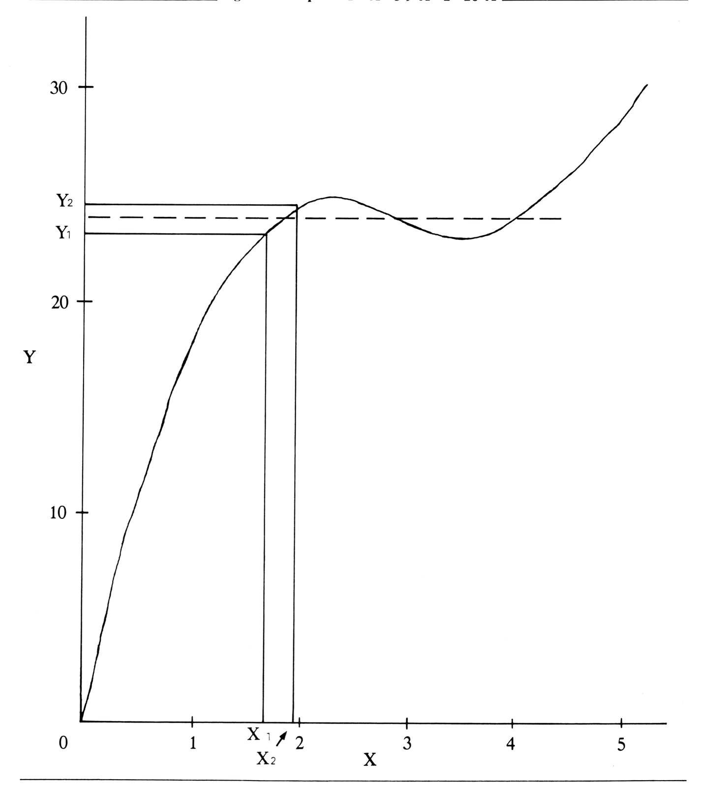
The method for doing this is called Linear Interpolation. Look at Figure 1 for a moment. Suppose that the solid curve shows the relationship between X and Y and that the dotted line indicates the value of Y that you are interested in. The value of X that yields this Y is found, of course, right beneath the point at which the dotted line hits the curve—somewhere between X1 and X2.

So select X1 and X2 as first approximations, find what values of Y1 and Y2 they correspond to, and then go for another estimated value of X according to what Y1 and Y2 tell you. The adjustment in X will not be strictly proportional to the error in Y unless the curve is a straight line in this region, but a proportional correction will still get you closer than you were, although on rare occasions you will come across a function that defies solution this way. Then use the new value of X as the approximate solution, and go through the process again, and again, if necessary, until you have reached the degree of accuracy you want.

Choosing your first X1 and X2 so that Y1 and Y2 surround the value is not usually imperative, but this can be helpful. In most cases, any two arbitrary approximations (as long as they are equal to each other) will suffice although some take longer to run than others.

Listing 1 contains the program to use. Type it in; press RUN and ENTER. The computer will ask you to enter the statement of the equation as Line 40. For example, the equation cited above would be entered as

40 LET Y=X**2+2*X

Then RUN 60 as the program instructs. The computer then tells you to enter a couple of guesses for X, as well as the target value for Y.

Then, as instructed, enter some tolerance figure to define the degree of accuracy that you want in the answer. Be realistic. If you ask for 0 tolerance, the computer will run all night seeking the impossible. If you specify 10% the computer will probably come a lot closer than 10%. If you call for .01%, the error seems usually to fall in the range of .001% or less. This is close enough for most practical purposes. In fact, you may want to “hard-write” (as an analogy with “hard-wire”) a tolerance limit of .01% or .001% instead of entering it each time.

Listing 1. Implicit Functions (8K ROM).

  10 PRINT "ENTER "" 40 LET Y=F(
X)"""
  20 PRINT
  30 PRINT "THEN RUN 60"
  50 RETURN
  60 PRINT
  70 PRINT "ENTER Y"
  80 INPUT Y0
  90 CLS
 100 PRINT
 110 PRINT "ENTER FIRST APPROXIM
ATION TO X"
 120 INPUT X1
 130 CLS
 140 PRINT
 150 PRINT "ENTER SECOND APPROXI
MATION TO X"
 160 INPUT X2
 170 CLS
 180 PRINT
 190 PRINT "ENTER TOLERANCE IN P
ERCENT"
 200 INPUT T
 210 CLS
 220 PRINT
 230 LET X=X1
 240 GOSUB 40
 250 LET Y1=Y
 260 LET X=X2
 270 GOSUB 40
 280 LET Y2=Y
 290 LET X3=(X1-X2)*(Y0-Y2)/(Y1-
Y2)+X2
 300 LET X1=X2
 310 LET X2=X3
 320 IF ABS (100*(X1-X2)/X1)>T T
HEN GOTO 210
 330 PRINT "X = ";X2

Limitations

This technique has one limitation that may be serious in some instances. Many equations have two or more solutions, but this approach will give you only one of them. In the example given, the two solutions are: X = 3 and X = -5. In the practical cases, you are interested only in the positive values since it is rather difficult to lay off a length of -5 feet. And, if you started out with positive values for your approximations to X, the computer will give you the positive answer, but you run into trouble if more than one solution is realistic.

The curve shown in Figure 1, for example, represents the equation Y = X ** 3 – 9 * X ** 2 + 26 * X. If Y = 24, the equation has three positive roots: 2, 3, and 4. This routine will give one or another of them according to the approximate values chosen as the points of departure. If it were not for this factor, entering “hard-write” values for X1 and X2 in lines 120 and 150 would be tempting.

Another caution: do not make your first approximations too small. Above all, do not use zero. Even if you expect your answer to be zero, it is better to start with numbers like 1 or 2 to reduce the possibility of running into numbers too big for the computer to handle in line 260.

One other danger to watch out for is in the handling of negative numbers. Remember that the ZX81 is not able to raise negative numbers to powers. I suspect that this is so because the computer uses logarithms in the process, and the logarithm of a negative number baffles computer and human alike. If this danger appears to be imminent, it can be avoided by the following substitutions:

For even-numbered exponents, replace X ** n by (ABS X) ** n.

For odd-numbered exponents, replace X ** n by SGN X * (ABS X) ** n.

Remember that it is very, very likely that you will run into negative numbers when you use trigonometric functions. The same strategem will work with them.

For even-numbered exponents, use (ABS (SIN X)) ** n.

For odd-numbered exponents, use SGN (SIN X) * (ABS (SIN X)) ** n.

The program can be translated to the 4K ROM by making the following change:

10 PRINT “ENTER#”;CHR$(212);”#40 LET Y=F(X)”;CHR$(212)

However, the program will lose some of its appeal because of the lack of floating point arithmetic. The answers will be in whole numbers so the closeness of the approximations will be lost.

One final limitation is that this routine will not give imaginary roots, i.e., square roots of negative numbers, designated by mathematicians as i and by engineers as j. But you have little chance of running into these unless you are working with AC power or electronic circuits.

One final caution, remember that the ZX81 gives you the arguments of trigonometric functions in radians. If you want degrees, multiply the radian value by 180/PI. (Ed.—See the article “Degrees, Grads, and Radians” elsewhere in this issue.)