Lissajous

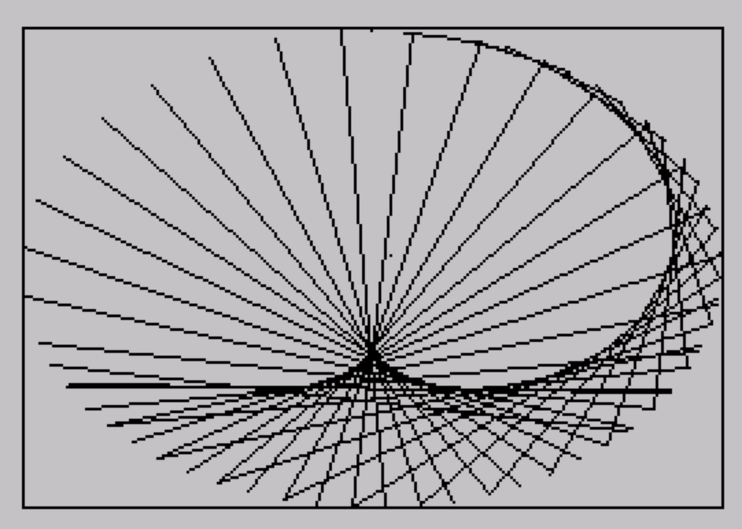
This program draws Lissajous figures on screen using parametric equations driven by a loop variable. The X coordinate is computed as 127·sin((m+1)·a)+127 and the Y coordinate as 87·cos((n+1)·a)+87, where m and n both equal 1/w and w increments each iteration, causing the frequency ratio to shift continuously. A border rectangle is drawn first using DRAW commands, and then each frame plots a line segment between consecutive points on the parametric curve. The program saves itself with an auto-run line using SAVE “LISSAJOUS” LINE 5.

---

Program Analysis

Program Structure

The program is organized into a short initialization block followed by a single drawing loop. Line 5 sets colors and clears the screen. Lines 10–20 initialize the frequency ratio variables. Lines 120–140 draw a border rectangle and set up the angle accumulator. Lines 210–350 form the core drawing loop, and line 360 jumps back to line 200, which does not exist — this causes the interpreter to resume at the next available line, which is 210, effectively looping continuously.

Parametric Curve Mathematics

The program implements Lissajous figures using the standard parametric form:

• x1 = 127·SIN((m+1)·a) + 127
• y1 = 87·COS((n+1)·a) + 87

Here m and n are initialized to 1/w (with w=1, so initially 1.0), and w increments by 1 each iteration of the outer loop. This causes the ratio between the sine and cosine frequency arguments to change continuously, producing an evolving series of Lissajous patterns rather than a static figure.

Coordinate Mapping

The offsets of 127 and 87 center the curves in the screen’s pixel space. The screen is 256 pixels wide and 176 pixels tall, so the amplitude factors (127 and 87) nearly fill the display area while the additions center the origin. The border is drawn at lines 120–120 using four chained DRAW commands from pixel origin (0,0).

Drawing Technique

Rather than plotting individual pixels, the program computes two successive points on the curve — (x1,y1) using (m+1)·a and (x2,y2) using m·a — then draws a line segment between them using PLOT x1,y1: DRAW x2-x1,y2-y1. This produces a connected curve rather than a dotted scatter plot, at the cost of two full parametric evaluations per step.

Notable Techniques and Anomalies

• The GO TO 200 on line 360 targets a non-existent line, causing execution to fall through to line 210 — a well-known BASIC technique to skip re-initialization on each loop iteration.
• LET m=1/w: LET n=m on line 20 ensures m and n are always equal, meaning the X and Y frequency arguments differ only by the constant offset of 1 in (m+1) vs. m.
• The angle step of 0.1 radians provides reasonable curve resolution; finer steps would slow drawing noticeably given the floating-point cost of two SIN/COS evaluations per iteration.
• Line 140 executes PLOT 134,92 (approximately the screen center) before the loop, which has no visible effect since subsequent PLOT calls in the loop override the graphics cursor immediately.

Variable Summary

Variable	Role
w	Incrementing counter controlling frequency ratio
m, n	Frequency ratio (always equal to 1/w)
a	Parametric angle accumulator, incremented by 0.1 each step
x1, y1	First point on curve (using (m+1)·a)
x2, y2	Second point on curve (using m·a)