

Good morning, Class! Today’s session will be on data point graphs. In the December 1982 issue, we discussed creating graphs on the screen that would show data points with connecting lines. The original program routine that created this was limited in the respect that only 12 sales entries could be entered. The screen was divided into 2 sections in which the left section of 8 columns was for data identification and the right 24 columns would contain the plotted graph.
Since each column can contain 2 subcolumns for the points being plotted, the routine would have three columns between points to use for connecting lines so that the graph could be easily visualized. This of course made for limited entry of only 12 data items.
It is possible to have as many as 64 data items entered but I decided to write a routine that would allow 24 entries and use only one sub-column for connecting lines. This program is at the end of this text.
The lines from 10 to 80. allow up to 24 data entries with line 40 terminating entry if the amount is less than 24.
The lines from 100 to 150 determine which entry is the largest so that the graph, when displayed, will have the highest peak at the very top of the screen down to zero sales at the bottom of the screen.
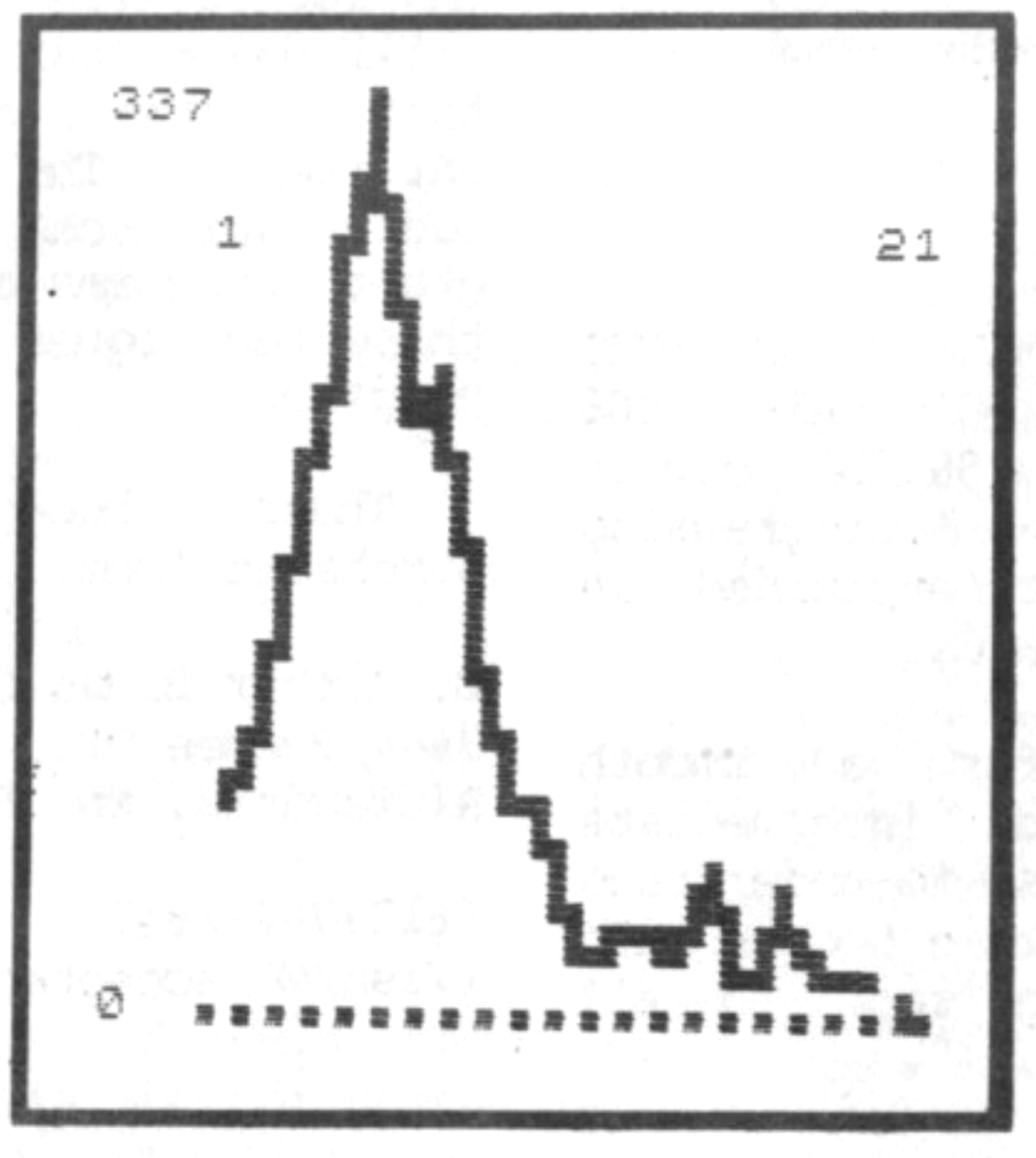
The lines from 200 to 630 PLOT the actual graph with the cubes at the bottom designating the division markers of the individual entries. The highest sales entry will be at the upper left of the screen and the entries from 0 to the total will be on the third line.
Subroutine 300 will plot the data points when they are going up and subroutine 400 will plot the data points when they are going down.
Subroutine 500 will plot the points to connect the data points when going up and subroutine 600 will plot the points to connect the data points when going down.
The sample graph shown on the cover represents a close approximation of sales of the ZX/TS 1000 series computers, starting in August of 1982 to present.
10 DIM S(24)
20 FOR N=1 TO 24
30 INPUT S(N)
40 IF S(N)=0 THEN GOTO 80
50 SCROLL
60 PRINT N,S(N)
70 NEXT N
80 LET R1=N-1
100 LET A=0
110 FOR N=1 TO R1
120 IF S(N)>A THEN LET A=S(N)
130 NEXT N
140 PRINT AT 21,1;0;AT 1,1;A
150 CLS
200 FOR N=4 TO R1*2 STEP 2
210 LET Y=(S(N/2)/A)*43
215 IF C=4 THEN GOTO 230
220 PLOT N+2,Y
230 GOSUB 300
240 PRINT AT 21,N/2+1;
    CHR$(4)
250 NEXT N
260 PRINT AT 3,3;1;AT 3,R1+1
    ;R1;AT 0,0;A;AT 21,0;0
270 PAUSE 40000
280 CLS
290 GOTO 200
300 LET Z=(S(N/2+1)/A)*43
310 IF Z<Y THEN GOTO 400
320 LET X=Z-Y
330 FOR C=1 TO 3
340 GOSUB 500
350 PLOT N+C+2,Y+C*X/3
360 NEXT C
370 RETURN
400 LET X=Y-Z
410 FOR C=1 TO 3
420 GOSUB 600
430 PLOT N+C+2,Y-C*X/3
440 NEXT C
450 RETURN
500 FOR D=Y+((C-1)*X/3)
    TO Y+((C)*X/3)
510 PLOT N+C+2,D
520 NEXT D
530 RETURN
600 FOR D=Y-((C-1)*X/3)
    TO Y-((C)*X/3) STEP-1
610 PLOT N+C+2,D
620 NEXT D
630 RETURN
Class dismissed!
Note: Type-in program listings on this website use ZMAKEBAS notation for graphics characters.